Are we really tilting?
The mechanics of reward guidance in flow and diffusion models
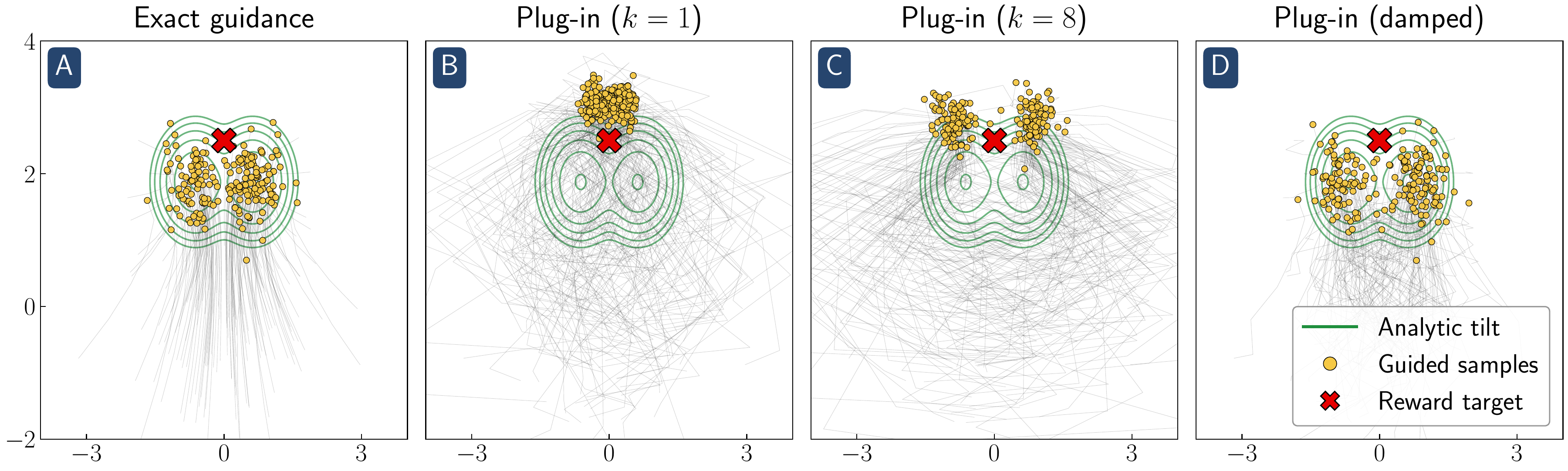
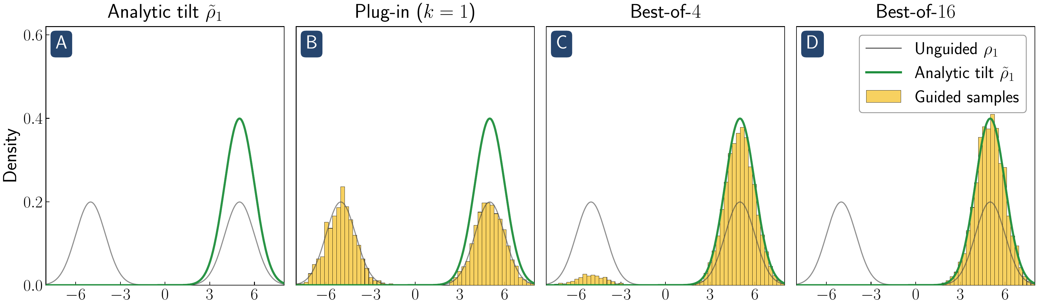
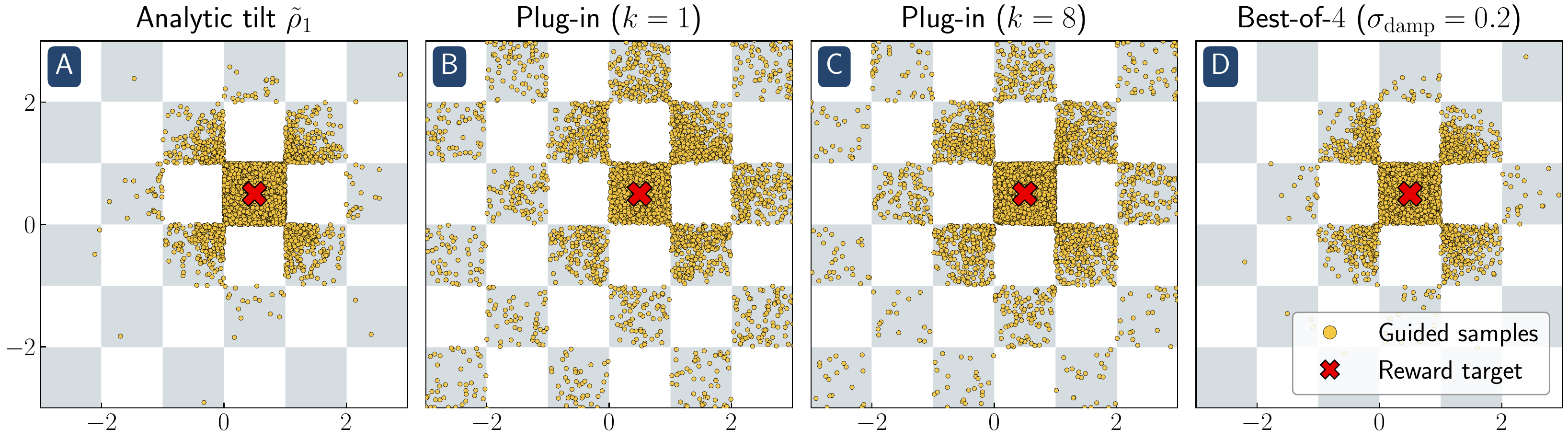
Reward guidance algorithms steer a learned generative process toward the reward-tilted measure at inference time. While empirically powerful, these methods are prone to reward hacking: the guided model over-optimizes the reward at the cost of fidelity to the learned distribution. We show that reward hacking arises from an approximation made in most practical implementations of reward-guided diffusion — finite-particle plug-in estimation of the Doob $h$-function — even in the simplest non-trivial settings of Gaussian and Gaussian-mixture targets with quadratic rewards. In closed form, we isolate two distinct failure modes: within-mode reward hacking and the inability to select high-reward modes. We propose a closed-form reward damping schedule that corrects the within-mode bias with no additional compute, and clarify the role of best-of-n sampling in fixing mode selection. Experiments on Gaussian mixture targets, a 2D checkerboard, and FLUX.1 text-to-image generation confirm that our theoretical insights carry over to practical settings.
“line of dogs of different breeds, with each dog taking on a color of the rainbow to form a technicolor gradient”
 Unguided
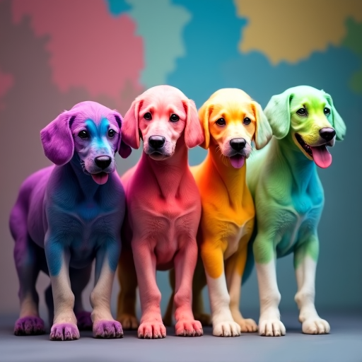 Guided
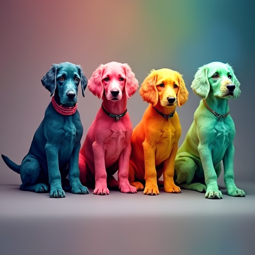 Damped (ours)
“stylized stop-motion scene of paper astronauts repairing a torn moon backdrop”
 Unguided
 Guided
 Damped (ours)
“renaissance painting of a sculptor in an open-air studio working on a headless statue”
 Unguided
 Guided
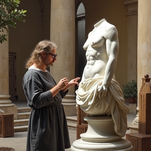 Damped (ours)
“editorial photo of a skyscraper under construction, missing its middle third”
 Unguided
 Guided
 Damped (ours)
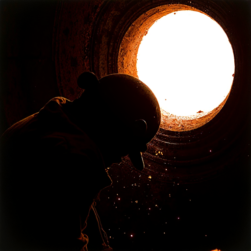
“brass automaton praying to a human child in an abandoned temple”
 Unguided
 Guided
 Damped (ours)
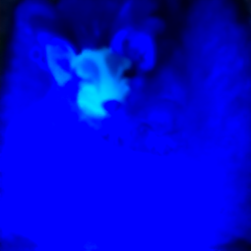
“koi pond full of vibrant fish, with the surface reflecting a mother and daughter looking down”
 Unguided
 Guided
 Damped (ours)