Deep reinforcement learning to play Ashta Chamma
June 25, 2023
This is a brief paper written by myself and Kason Ancelin (UCLA) for our final project in CS 260C (grad. deep learning). We used deep-Q learning with experience replay to train an agent to play Ashta Chamma, a board game that I play with my grandmother in India. Ashta Chamma is somewhat similar to Sorry, Ludo, or Trouble (if you’re familiar with those games). All of the code that we wrote can be found in the associated repository on GitHub. You can run the play.py file on your local machine to play against any of our preset policies or the final trained deep reinforcement learning agent.
Background
Q-learning is a reinforcement learning algorithm that enables an agent to learn optimal actions in a Markov decision process (MDP) environment through trial and error. At its core, Q-learning utilizes a value function called the Q-function (sometimes referred to as the Q-table), which represents the expected long-term cumulative reward of taking a particular action in a given state. The Q-function is updated iteratively based on the observed rewards obtained from the agent’s interactions with the environment. We typically establish these rewards before training. By learning the optimal Q-values for each state-action pair, the agent can make informed decisions to maximize its expected cumulative reward over time.
The Q-learning algorithm follows a simple iterative process to update the Q-values. Initially, the Q-values are randomly initialized for all state-action pairs. The agent then selects an action based on an exploration-exploitation trade-off strategy, which can involve either selecting the action with the highest Q-value (exploitation) or randomly exploring other actions (exploration). This is typically controlled by a parameter $\epsilon$; with probability $\epsilon$ a uniformly random action will be chosen to explore the environment. Typically, $\epsilon$ decays as training progresses in order to transition from exploration of the environment to exploitation of existing knowledge.
After performing the selected action, the agent observes the resulting state and the reward associated with the transition. The Q-value of the previous state-action pair is updated using the observed reward and the maximum Q-value of the next state. This update is performed iteratively for each interaction, gradually refining the Q-values until we get convergence to the optimal values. Below is a condensed form of this algorithm:
- Initialize Q-values.
- Choose action $a$ for state $s$ (selection based on highest Q-value).
- Perform action $a$, get new state $s^\prime$.
- Observe reward $R$.
- Update Q with the Bellman equation ($Q_{\text{new}} = \mathbb{E}[R_{t+1} + \gamma \max_{a^\prime}\ q(s^\prime, a^\prime)]$).
- Repeat steps 2 through 5 until desired performance is achieved.
Deep Q-learning builds upon the principles of Q-learning by incorporating deep neural networks to handle high-dimensional state spaces. Traditional Q-learning struggles with complex environments due to the exponential growth of the state-action space. Deep Q-learning addresses this challenge by utilizing a deep neural network as a function approximator to estimate the Q-values. Through training, the neural network takes the current state as input and learns to output a Q-value for each possible action. By leveraging the capabilities of deep learning, the agent can learn meaningful representations of the environment and make accurate predictions.
Deep Q-learning employs an experience replay mechanism to stabilize the learning process and improve sample efficiency. Instead of updating the neural network after every interaction, the agent stores the observed experiences in a replay buffer. During the learning phase, a mini-batch of experiences is randomly sampled from the replay buffer to update the network. This approach decouples the dependencies between consecutive experiences and allows the agent to learn from a diverse set of transitions (due to the exchangeability of the samples). By combining the power of deep neural networks with the iterative Q-learning algorithm and experience replay, deep Q-learning has demonstrated impressive results in various challenging tasks. Here’s the deep Q-learning algorithm written explicitly:
- Initialize Q-values.
- Choose action $a$ for state $s$ (selection based on highest Q-value).
- Perform action $a$, get new state $s^\prime$.
- Observe reward $R$.
- Update weights for the deep Q-network using backpropagation.
- Repeat steps 2 through 5 until desired performance is achieved.
Notice that the only distinction between the the Q-learning and deep Q-learning algorithm is the update step, in which Q-learning uses the Bellman equation and deep Q-learning updates the weights of a neural network. This is precisely the point of deep Q-learning: to use a neural network to learn the Q-function which is significantly more scalable and learns to approximate Q-values as opposed to calculate them via the computationally expensive Bellman equations.
Rules
Ashta Chamma is a game that I play with my grandmother in India. Here’s a picture of the initial setup of the board:
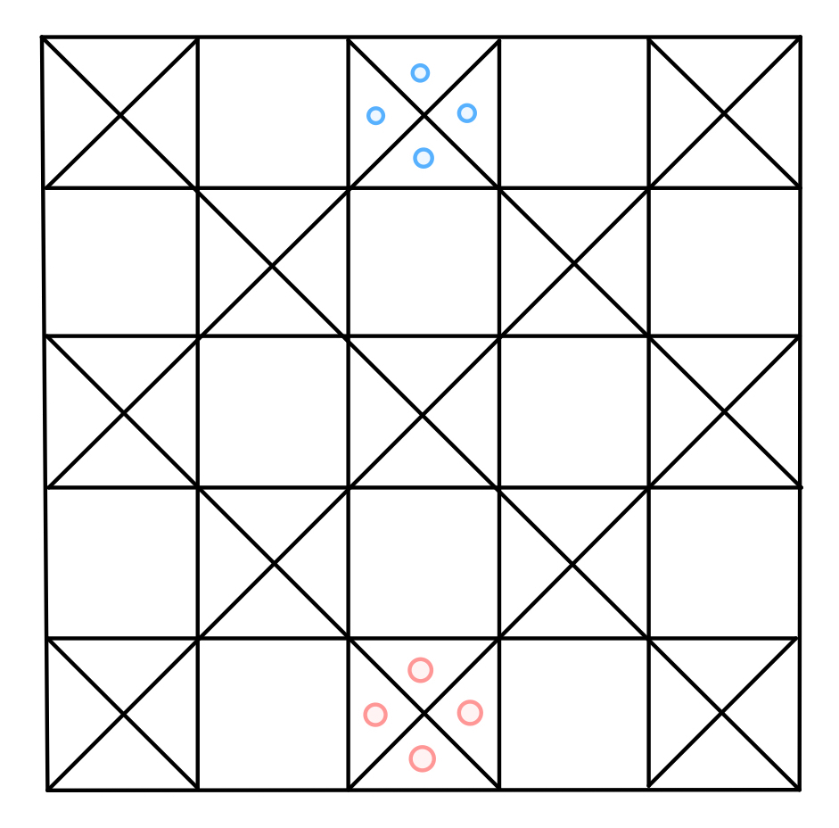
Initial setup of the Ashta Chamma game board
The goal is to move all your pieces into the center. On your turn, you roll four cowry shells (which can either land face-up or face-down):

Cowry shells rolled in Ashta Chamma to determine move
The number of face-up shells corresponds to the number of moves you make (where all four shells face-down represents 8). If you roll a 4 (“chamma”) or an 8 (“ashta”), you must roll again. The path that your pieces take is depicted below:
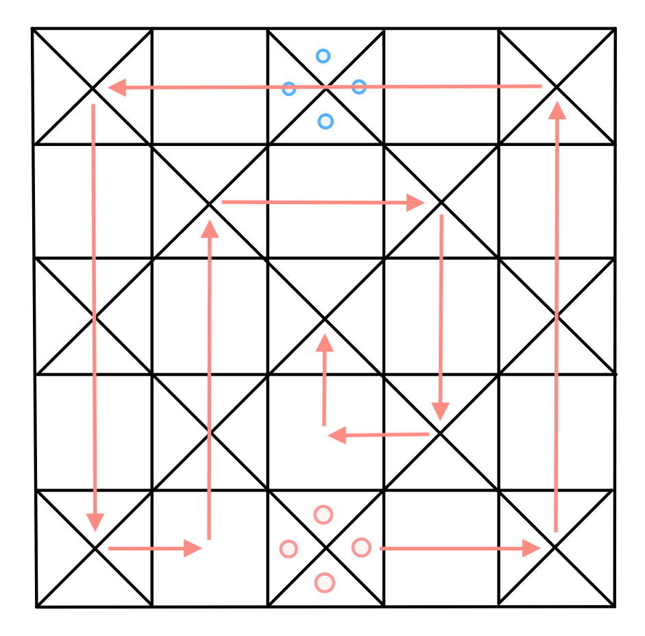
Path that pieces take on an Ashta Chamma board
On your turn, you can choose one piece to move forward with the number of moves corresponding to your roll. The squares marked with an “X” are safe squares and any number of pieces can be on a safe square at a time. You are not allowed to move your piece onto another one of your pieces on a non-safe square. Moving onto an opponent’s piece on a non-safe square moves the opponent’s piece back to start (a “capture”) and you must roll again. You are not allowed to move any pieces past the end of the board. If there is no legal move for you to make, you forfeit your turn. Additionally, you are not allowed to move past the safe square on the left-hand side until you have made a capture.
The goal of the agent is to learn which piece to move in order to win the game. The first step for our project was to subclass the Farama Foundation’s gymnasium environment to implement the rules of the game. More precisely, on the agent’s turn, the game’s environment is responsible for moving a piece, handling the opponent’s turn, rolling the shells, and relinquishing control back to the player. However, there were several edge cases which made this task difficult. For example, if the player rolls an 8 and has no legal follow-up moves, the game must remember and revert back to its original state. Therefore, the task of implementing the game rules became much more involved than we originally anticipated, and it became an exercise in software engineering to create a robust and bug-free environment.
Internally, the game state is represented as a dictionary containing the current roll, positions of both players’ pieces, flags representing whether each player has made a capture yet, and a remembered state in case of a multi-turn move. The probabilities for the shells are taken from previous work written studying pure strategies for playing Ashta Chamma without AI. The environment contains a function to_array which concatenates the state into a one-dimensional numpy array. The code for the environment can be found in the env.py file in our GitHub repository.
Policies
While training the agent to play the game, we had to create policies for the model to train against; these dictate how the agent’s opponent will play during training. We wrote the following policies and trained the network against each of them several times. For the policies described below, the word “randomly” is used to describe random selection that is taken uniformly across possible moves.
- Random policy: Randomly selects a move among the possible legal moves.
- Offense policy: If one of its possible moves captures an opponent’s piece, it takes this move. Otherwise, it randomly selects a move.
- Safe policy: If one of its possible moves places one its pieces on a safe space, it takes this move. Otherwise, it randomly selects a move.
- Smart policy: If one of its possible moves captures an opponent’s piece, it takes this move. Otherwise, it randomly selects a move.
- Fast policy: Always moves the furthest ahead piece with a possible legal move.
- Slow policy: Always moves the furthest behind (closest to start) piece with a possible legal move.
Training
The deep Q-network (DQN) constructed to train the agent’s policy is a 3-layer deep fully-connected neural network which accepts the inputs as a 1-D tensor, has 128 neurons in each hidden layer, and has 4 output neurons (each representing a possible move in the game). Between each layer is a ReLU activation; however, we did experiment with different neural network architectures and parameters. When experimenting with a convolutional neural network via the nn.Conv1d layer in PyTorch, we found no significant improvement of the network’s performance against its linear-layered counterpart.
Furthermore, we also trained deeper network architectures with 3-5 hidden layers on on both fully-connected networks and convolutional networks. The performance of these networks did not exceed the performance of the 3-layer deep fully-connected network described above. Since the experimentation described above achieved similar or worse performance using a significantly more complicated model, we chose to train the simpler model, which we found was still quite expressive. This is in the interest of avoiding over-training since the game’s complexity may not warrant the complexity of these alternative networks. In addition, the training speed of the linear network was much faster, which allowed us to allow the agent to play more samples.
Another observation made during hyperparameter tuning was the importance of weight and bias initializations. Training runs with the same hyperparameters and network often returned different performance results and statistics. For instance, identical training runs (except for weight and bias initializations) of the agent against the smart policy yielded between a 30% and 55% win rate on the second run. In particular, we found that weight initializations and the initial random exploration when $\epsilon$ is large have a very significant effect on the overall performance of the model. Therefore, we chose to use a genetic-style training algorithm, wherein we trained the model for 500 episodes at a time against various models. For each iteration, we would run the model against the same policy five times, keeping the best results. We found that training the model against a variety of policies yielded the best performance. After 17 iterations of this genetic-style algorithm, we were able to create a state-of-the-art model.
Training was done with the Adam-W optimizer and the final results displayed in this paper resulted from a network whose training procedure used a batch size of 8, $\gamma = 0.999$, $\epsilon_{\text{start}} = 0.95$, $\epsilon_{\text{end}} = 0.05$, $\epsilon_{\text{decay}} = 500$, $\tau = 0.005$, and a learning rate of $1 \cdot 10^{-5}$, and for 500 episodes for each iteration of the genetic-style algorithm. The full training loop procedure and model evaluation can be found in \ci{train.py} file located on the project’s GitHub repository. \par We settled on rewarding the agent +1 point for a win, -1 for a loss, and 0 points for a draw (when neither player can make any legal moves). In combination with the network and training procedure, we found this intuitive reward system yielded the best results.
Results
Below are some plots depicting the running average win rate over the course of our training process. Note that the average win rate is highly irregular at the start of training due to the high $\epsilon$-value, which corresponds with the model trying random moves and exploring the environment. The three figures below display the agent’s running average win rate during training against the random, fast, and offense policy, respectively. The plots display the agent training and receiving quite impressive results including a 80% winning rate against the random policy and a 75% winning rate against the offense policy.
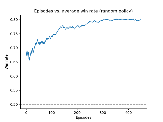
Running average win rate of the deep Q-network training against the random policy
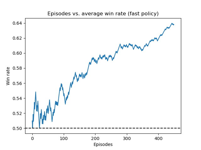
Running average win rate of the deep Q-network training against the fast policy
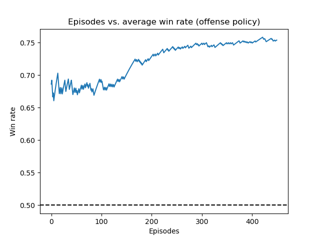
Running average win rate of the deep Q-network training against the offense policy
Upon training an agent which could effectively play against the above policies, we trained the agent to play against the most sophisticated and competitive policy: the smart policy. The results of this experimentation are displayed below in the two below figures:
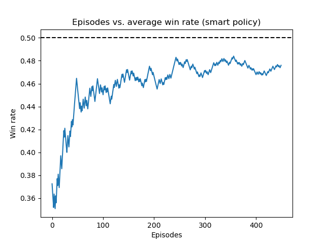
Running average win rate against smart policy (before genetic-style training)
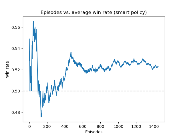
Running average win rate against smart policy (after genetic-style training)
Notice that in the first figure the model did not achieve a high win rate and was in fact still losing more often than it won against the strategy. However, we included this graph to display how significantly the agent learned to become competitive against this strategy through the training process. The second figure displays the best accuracy achieved against the smart policy, after 17 iterations of repeated genetic-style training against all of our policies. We see that the agent learns to beat the smart strategy in this case and is able to achieve a final win rate of around 52.5%.
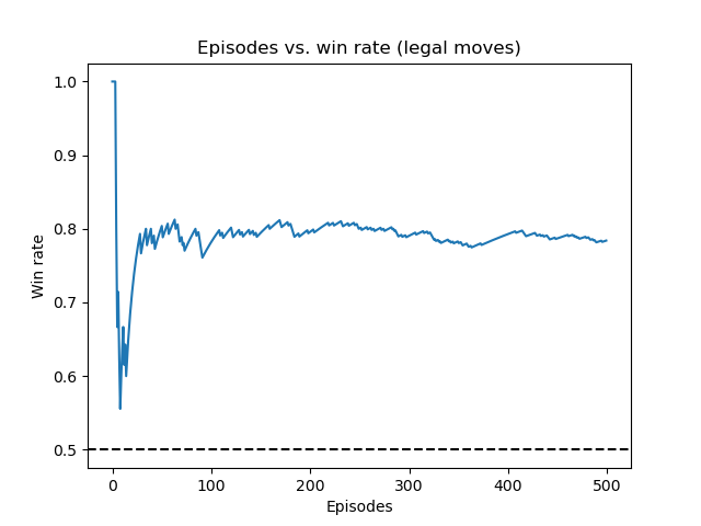
Running average win rate against random policy (after genetic-style training)
Contrarily, the above figure shows the agent training against the random policy after genetic-style training and achieving a stable accuracy rate extraordinarily fast with very few episodes. Therefore, this pre-trained agent generalizes extraordinarily well to playing opponents employing other strategies.
Finally I played a few games against the model myself as a heuristic test and the agent was able to play competitively against me. The agent simultaneously played aggressively (capturing whenever possible) and conservatively (landing on safe squares whenever possible). In addition, the agent did not move pieces into squares where they were likely to be captured. Overall, I was quite impressed by the model’s performance.
Conclusion
With relatively little computing power, we were able to train an agent to win at least 70% of games against all programmed policies (excluding smart) and upwards of 85% against the random policy. The best previous work we could find studying the Ashta Chamma game achieved a win rate of 56% (without using artificial intelligence) against three other random policies in a four-player version of the game. In particular, the win rates we were able to achieve using deep Q-learning are state-of-the-art for the two-player game and our agent was able to beat the policies described in this paper.
Against the smart policy, the agent developed a policy which yielded a 52.5% win rate. This win rate is likely because the smart policy is close to optimal already and we simply did not have the computational resources and time to hyperparameter tune the DQN to achieve a higher win rate. We believe that with more computational resources and time, we could achieve a higher win rate against the smart policy. Future modifications of this work could include training on even more complicated policies, training against an opponent whose policy is chosen randomly at each iteration, or training against the model itself. As the level of play of the opponent policy increases, we will need more computational resources to accommodate training against the more complicated strategies.
In summary, our implementation of the Deep-Q learning algorithm succeeded in learning how to play Ashta Chamma at a high level and beat opponents of various strategies, but there is more work that can be done to improve the current agent’s performance.
The version of Ashta Chamma implemented here is a very slightly simplified version of the game. While there is variety in how Ashta Chamma is played by different people, another potential extension would be to incorporate all of the rules used in the original form of Ashta Chamma that I play with my family. For example, rolling three or more 8’s in a row invalidates all three 8’s. Furthermore, it should actually be possible to move past the pre-capture boundary if you are doing so in order to capture a piece. Finally, if you roll a 4 or 8 and simultaneously capture a piece, this should actually give you two extra turns (and not one). Yet another extension would be to allow the algorithm to play against three other players and not just one (in the four-player version of the game).