The Mapper algorithm for topological data analysis (TDA)
July 17, 2023
In this note, I’ll discuss some of the ways in which differential geometry can be applied to study the topological features of a dataset. We’ll discuss some of the fundamental concepts behind topological data analysis (TDA), and my goal is to provide an exposition to the Mapper algorithm, the most commonly-used TDA algorithm.
We want to know which parts of the data are “connected”, and in what way the points in the dataset are related. In particular, we would like to know how the dataset is distributed and we would like to use the patterns we find to classify our data. However, we want to ignore certain spatial aspects of the data, such as the density of the points and the shapes they create. This is an unsupervised learning model, meaning that we can use it on unlabeled data points; all relevant insights will be generated by the algorithm.
Background
We’ll start by defining a few terms and providing some of the background for the Mapper algorithm. Suppose $(X, \rho)$ is a metric space. Then, we’ll define a dataset to be a finite point cloud $D \subseteq X$. Also, recall that an open cover $\mathcal{G}$ of $S$ is a set $\lbrace G_i \rbrace_{i=1}^n$ such that $G_i$ is open for all $1 \leq i \leq n$ and $S \subseteq \bigcup_{i=1}^n G_i$. Furthermore, a filter (or lens) is a continuous function $f : X \to \mathbb{R}^d$; for the purposes of this note, we’ll be looking at the case wherein $d = 1$ and $f : X \to \mathbb{R}$.
Now, suppose $f$ is a filter and $\mathcal{G}$ is an open cover for the image $f(X)$. Then, the pullback of $\mathcal{G}$ under $f$ is $\lbrace f^{-1}(G_i) \rbrace_{i=1}^n$, which is also an open cover for $X$. Note that $f^{-1}(G_i)$ is open for all $1 \leq i \leq n$ since continuous preimages of open sets are open. Also, for all $x \in X$ we have $f(x) \in f(X) = \bigcup_{i=1}^n G_i \implies x \in \bigcup_{i=1}^n f^{-1}(G_i)$ by definition so the pullback is indeed an open cover. Then, the refined pullback of $\mathcal{G}$ under $f$ is the set $\mathcal{C}$ of connected components of the pullback of $\mathcal{G}$ under $f$. Essentially, taking the refined pullback will split $f^{-1}(G_i)$ into its various connected components for all $i$.
We’re ready to define the nerve by the undirected graph $(V, E)$ given by $V = \mathcal{C}$ where $(C_i, C_j) \in E$ if and only if $i \neq j$ and $C_i \cap C_j \neq \varnothing$. But why do we care about the nerve?
The nerve theorem from topology states that if $\mathcal{C}$ is an open cover for a topological space $Y$ and the intersection of any two elements of $\mathcal{C}$ is contractible (can be shrunk to a point) then the nerve $N(\mathcal{C})$ is homotopy-equivalent to $Y$. In particular, we can always deform the nerve in some way to get $Y$ back. This means that the nerve gives us very valuable topological information about a space, which is exactly what we set out to study!
In fact, we can generalize the notion of a nerve to higher dimensions. The abstract simplicial complex associated to a vertex set $V$ is $V \subseteq K \subseteq \mathcal{P}(V)$ such that for any element $k \subseteq K$ we have all subsets of $k$ also contained in $K$. In this case, the elements of $K$ are called faces or simplices. We can define the dimension of a simplex $\dim(k) = \lvert k \rvert - 1$; this makes sense geometrically. Recall that a simplex is the generalization of the notion of a triangle, and a triangle contains three points but has dimension two.
Notice that a simplex of dimension one is just an undirected graph with vertex set $V$; it must contain $V$ along with sets containing two elements of $V$ (these will be the edges). In fact, we can define the nerve more generally for a higher-dimensional filter function $f : X \to \mathbb{R}^d$ using an abstract simplicial complex instead of a graph. However, this is outside the scope of what I want to discuss with this note.
The Mapper algorithm
This is cool and epic. Now, we’re finally ready to talk about the Mapper algorithm (as described in this paper)! Our goal is to study a dataset $D$ using the refined pullback of some open cover of $f(D)$, and the Mapper algorithm described below does precisely that.
Mapper Algorithm [Singh et al., 2007].
- Take as input a metric space $(X, \rho)$, a dataset $D \subseteq (X, \rho)$, a filter function $f : X \to \mathbb{R}^d$, and an open cover $\mathcal{G}$ of $f(D)$.
- For each $G_i \in \mathcal{G}$ decompose $C_i = f^{-1}(G_i)$ into clusters ${ C_i^j }_{j=1}^m$ using your favorite clustering algorithm ($k$-means, spectral clustering, Gaussian mixture models, etc.). This will give us the equivalent of a refined pullback for a dataset (which is finite).
- Notice that $\mathcal{C} = { C_i^j }_{i, j}$ forms an open cover for $D$ and hence we can find where these sets intersect and compute the nerve $N(\mathcal{C})$.
- Output the nerve $N(\mathcal{C})$ (which will be a graph if $d = 1$ and a simplicial complex otherwise).
But how do we choose inputs to the Mapper algorithm? The most common way to choose a cover is to choose a resolution $r > 0$ and cover $f(D)$ with equally-spaced intervals $(a, b)$ of length $r$. In the more general case, we can cover $f(D)$ with Cartesian products of such intervals.
In addition, one common choice for the filter function is the centrality function $f(x) = \sum_{y \in D} \rho(x, y)$. Another common choice for the filter function is the eccentricity function $f(x) = \max_{y \in D} { \rho(x, y) }$. Each of these choices will give us different information about the dataset. Furthermore, if $X = \mathbb{R}^d$ then $f(x) = \operatorname{proj}_{v}(x)$ is called the height function and the output of the Mapper algorithm is called the Reeb graph. Since the height function is the easiest to visualize, we’ll provide some examples of the Mapper algorithm applied with the height function below.
Examples and applications
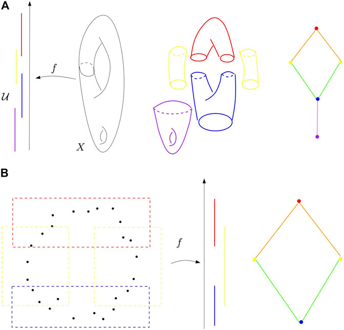
The following is a diagram taken from a paper by Frédéric Chazal and Bertrand Michel.

A diagram outlining the Mapper algorithm
In particular, consider the second example, wherein we have a finite dataset $D$. In this case, we use the height function to map $D$ into $\mathbb{R}$ and provide open cover for $f(D)$. Then, we take the pullback of each of these sets under $f$ and use a clustering algorithm to turn this into a “refined pullback” for our open cover of $f(D)$ under $f$. Then, we can compute the nerve using a union-find data structure (or something similar). Then, notice that the nerve does indeed give us valuable information about the topological structure of our original data (it has a hole in it)!
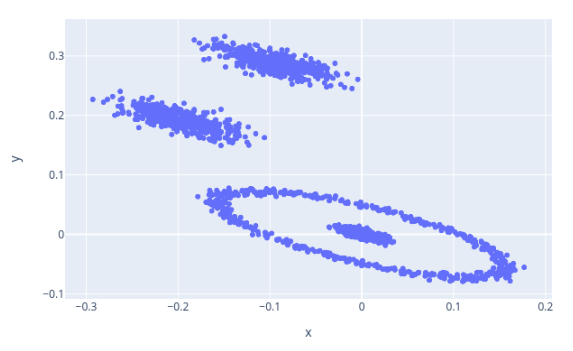
The following is the output of the Mapper algorithm on data generated by the sklearn package and embedded into $\mathbb{R}^2$ using the tadasets package by Daniel Edmiston.

A sample dataset showcasing the Mapper algorithm

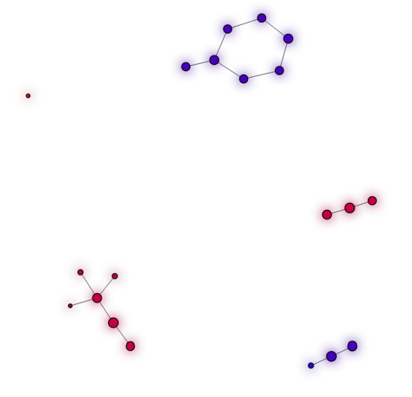
The output of the Mapper algorithm on the dataset shown above
Aside from the one extraneous dot on the left-hand side of the output, we find that our original dataset is composed of a loop and three separate clusters as desired. Notice that the Mapper algorithm does not tell us that one of our clusters is contained inside of the loop; this is not relevant to the fundamental topological structure of the dataset. Finally, we’ll discuss some applications of the Mapper algorithm. The Mapper algorithm has been used to:
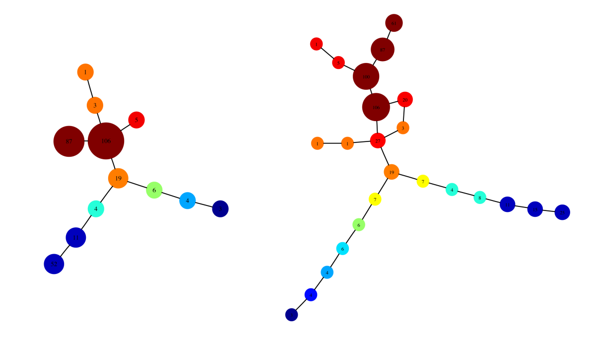
- Classify different kinds of diabetes and heart disease and make it easier to diagnose and treat patients (see the below image)
- Classify poses in 3D models of various animals created by illustrators and animators
- Estimate the Betti number of high-dimensional surfaces by sampling points from the surface

An application of the Mapper algorithm to analyzing data on diabetes risk factors
For example, in this image (from the original Mapper algorithm paper) we can see the output of the Mapper algorithm on a dataset containing risk factors for diabetes along with clinical diagnoses. The Mapper algorithm is able to clearly identify Type I and Type II diabetes (see the left and right branches respectively) and in fact can help diagnose the severity of diabetes that someone is likely to have (!). The fact that the topology of the dataset alone can tell us something profound about diabetes (without any knowledge of the relevant biology) is a very surprising and wonderful application of mathematics.