The optimality of Morris' algorithm
May 23, 2023
- Morris’ algorithm
- Fooling around
- Trick #1
- Trick #2
- Space complexity
- Extensions of Morris’ algorithm
- Generalizing the exponent
- Floating-point counters
- Counting chains
- Experimentation
- Proof of optimality
- Applications
Something I’ve been thinking about lately is my final project for Stats 200C at UCLA (grad. high-dimensional stats). The topic I chose is algorithms for approximate counting, which I found particularly interesting because I participated in an REU under Prof. Jelani Nelson last summer, who’s an expert in this field. In any case, here’s a cool counting algorithm I’ve been reading about (which is provably optimal).
Morris’ algorithm
Let’s start with the traditional Morris’ algorithm due to Robert Morris in 1978 at Bell Labs. We would like a data structure to count (approximately) up to a large number $n$ using very little storage - this is called the “approximate counting” problem. In exchange for the reduced space complexity, maybe we don’t need the exact count - we only need to get reasonably close. This data structure should support increment() and query() methods, to increment the count and return an estimate of the current count respectively. Typically, we would need $\log_2(n)$ bits in the worst case to naïvely count up to a number $n$.
One easy idea: what if we only incremented with probability $\frac{1}{2}$ each time? Then, maybe we could multiply our count by 2, and by the law of large numbers, we can expect a reasonably good estimator for the true count. However, we would still expect to need $\log_2(n) - 1$ bits to store the number. This still requires $O(\log(n))$ bits in expectation, but we can do better; this is the idea of Morris’ algorithm. As the count gets larger, we increment with smaller probability. Here’s an incomplete data structure reflecting this idea:
from random import getrandbits

class MorrisCounter:
    def __init__(self):
        # initialize the counter to 0
        self.counter = 0

    def update(self):
        # increment counter with probability 1/2^(counter)
        if not getrandbits(self.counter):
            self.counter += 1
A lot of these algorithms use dyadic probabililities (multiples of $\frac{1}{2^k}$ for $k \in \mathbb{N}$), since it’s typically faster to generate pseudo-random bits than to generate a pseudo-random floating point number in an interval like $[0, 1]$.
This is a good idea because $n \mapsto \frac{1}{2^n}$ decays quickly, so with high probability our estimator will be a relatively small number (we’ll quantify this later). But given this update algorithm, what should a query to the true count return? Define $X_n$ to be the count in Morris’ algorithm after $n$ updates. Then, we have by the law of total expectation:
\[\begin{align*} \mathbb{E}[2^{X_{n+1}}] & = \sum_{k=0}^\infty \mathbb{P}(X_n = k) \cdot \mathbb{E}[2^{X_{n+1}} \vert X_n = k] \\ & = \sum_{k=0}^\infty \mathbb{P}(X_n = k) \cdot \left( 2^{k+1} \cdot \frac{1}{2^k} + 2^k \cdot \left( 1 - \frac{1}{2^k} \right) \right) \\ & = \sum_{k=0}^\infty \mathbb{P}(X_n = k) \cdot (2^k + 1) \\ & = \mathbb{E}[2^{X_n}] + 1. \end{align*}\]Since $2^{X_0} = 2^0 = 1$, we know that $\mathbb{E}[2^{X_0}] = 1$. Solving the recurrence in $n$ gives $\mathbb{E}[2^{X_n}] = n + 1$, which suggests that $2^{X_n} - 1$ is an unbiased estimator for $n$. Therefore, we obtain the complete Morris’ algorithm:
from random import getrandbits

class MorrisCounter:
    def __init__(self):
        # initialize the counter to 0
        self.counter = 0

    def update(self):
        # increment counter with probability 1/2^(counter)
        if not getrandbits(self.counter):
            self.counter += 1

    def query(self):
        # return the unbiased estimate
        return (1 << self.counter) - 1
Using bit-shift operators like
1 << xinstead of built-in exponentiation operatorsmath.pow(2, x)or2 ** xis sometimes slightly faster.
Just how good is this estimator? Well, Chebyshev’s inequality tells us that $2^{X_n} - 1$ concentrates around its mean:
\[\mathbb{P}(\lvert 2^{X_n} - 1 - n \rvert \geq n \epsilon) \leq \frac{1}{\epsilon^2 n^2} \cdot \mathbb{E}[(2^{X_n} - 1 - n)^2].\]But we have:
\[\begin{align*} \mathbb{E}[2^{2 X_{n+1}}] & = \sum_{k=0}^\infty \mathbb{P}(X_n = k) \cdot \mathbb{E}[2^{2 X_{n+1}} \vert X_n = k] \\ & = \sum_{k=0}^\infty \mathbb{P}(X_n = k) \cdot \left( 2^{2k+2} \cdot \frac{1}{2^k} + 2^{2k} \cdot \left( 1 - \frac{1}{2^k} \right) \right) \\ & = \sum_{k=0}^\infty \mathbb{P}(X_n = k) \cdot (2^{k+2} + 2^{2k} - 2^k) \\ & = \mathbb{E}[2^{X_n + 2}] + \mathbb{E}[2^{2 X_n}] - \mathbb{E}[2^{X_n}] \\ & = 3 (n + 1) + \mathbb{E}[2^{2 X_n}]. \end{align*}\]Again, we can solve the recurrence with the initial condition $\mathbb{E}[2^{2 X_0}] = 1$ to find $\mathbb{E}[2^{2 X_n}] = \frac{3}{2} n^2 + \frac{3}{2} n + 1$. Therefore, we have (for $n \geq 1$):
\[\begin{align*} \mathbb{E}[(2^{X_n} - 1 - n)^2] & = \mathbb{E}[(2^{X_n} - (n + 1))^2] \\ & = \mathbb{E}[2^{2 X_n}] - 2 (n + 1) \mathbb{E}[2^{X_n}] + (n + 1)^2 \\ & = \frac{3}{2} n^2 + \frac{3}{2} n + 1 - 2 (n + 1)^2 + (n + 1)^2 \\ & = \binom{n}{2} \\ & < \frac{n^2}{2}. \end{align*}\]Therefore, our original Chebyshev bound gives:
\[\mathbb{P}(\lvert 2^{X_n} - 1 - n \rvert \geq n \epsilon) < \frac{1}{2 \epsilon^2}.\]This bound suggests that this algorithm is really not that great. In particular, we need $\epsilon \geq 1$ to at least get a failure probability better than $\frac{1}{2}$. But with $\epsilon \geq 1$, Chebyshev’s inequality only tells us (at best) that our estimate is in $[0, 2n]$. This is a really wide range, and not very useful at all.
Fooling around
Okay, so we have a not-so-great algorithm. But we’re computer scientists, and that isn’t going to stop us from trying to make this work! There are a few tricks we can use to sharpen our estimate.
Trick #1
We’ll create $s$ independent instantiations of the Morris algorithm and take an average to reduce the variance. Letting $\tilde{n}_i$ be the estimator given by the $i$th instantiation, our estimator is $\tilde{n} = \frac{1}{s} \sum_{i=1}^s \tilde{n}_i$. Then, by properties of variance and our previous result about Morris’ original algorithm:
\[\mathbb{E}[(\tilde{n} - n)^2] = \frac{1}{s} \cdot \mathbb{E}[(2^{X_n} - 1 - n)^2] \leq \frac{n^2}{2s}.\]Now, Chebyshev’s bound gives the sharper estimate:
\[\mathbb{P}(\lvert \tilde{n} - n \rvert \geq n \epsilon) < \frac{1}{2 s \epsilon^2}.\]Now, we can fix a failure probability $\delta > 0$ and choose $s \geq \frac{1}{2 \epsilon^2 \delta}$ so that $\mathbb{P}(\lvert \tilde{n} - n \rvert \geq n \epsilon) < \delta$. This algorithm is sometimes called “Morris+”.
Trick #2
Here’s another neat trick to further reduce the dependence of our bound on the failure probability $\delta$ from $\frac{1}{\delta}$ to $\log\left( \frac{1}{\delta} \right)$. Run $t$ instantiations of Morris+, each with failure probability $\delta = \frac{1}{3}$, for instance. Then, let $Y_i$ be 1 if the $i$th Morris+ algorithm fails and 0 otherwise, so that we get the following bound for free:
\[\mathbb{E}\left[ \sum_{i=1}^t Y_i \right] = \sum_{i=1}^t \mathbb{E}[Y_i] = \sum_{i=1}^t \mathbb{P}(Y_i = 1) \leq \frac{t}{3}.\]Then, since $0 \leq Y_i \leq 1$ is a bounded random variable (and therefore sub-exponential), Hoeffding’s inequality allows us to control the number of failures:
\[\mathbb{P}\left( \sum_{i=1}^t Y_i \geq \frac{t}{2} \right) \leq \mathbb{P}\left( \sum_{i=1}^t Y_i - \mathbb{E}\left[ \sum_{i=1}^t Y_i \right] \geq \frac{t}{6} \right) \leq \exp\left( -\frac{t}{18} \right).\]Choosing $t \geq 18 \log\left( \frac{1}{\delta} \right)$, we get $\mathbb{P}\left( \sum_{i=1}^t Y_i \geq \frac{t}{2} \right) \leq \delta$. In particular, this means that choosing $t$ this way, the median $\tilde{n}$ of the Morris+ runs satisfies $\lvert \tilde{n} - n \rvert < n \epsilon$ with probability at least $1 - \delta$. Therefore, we take the median of our Morris+ instantiations as our new estimator and obtain an improved failure rate. This algorithm is sometimes called “Morris++”.
Space complexity
Fix $\epsilon > 0$ and $\delta > 0$. Running Morris++ with the minimal choices of $s$ and $t$ requires running Morris+ for $t = \Theta\left( \log\left( \frac{1}{\delta} \right) \right)$ iterations, each of which require running the original Morris’ algorithm $s = \Theta\left( \frac{1}{\epsilon^2} \right)$ times. If any counter in the original Morris’ algorithm reaches $\log_2\left( \frac{nst}{\delta} \right)$, it will be incremented with probability at most $\frac{\delta}{nst}$. Therefore, a union bound tells us that the probability that the counter will be incremented in the next $n$ steps is at most $\frac{\delta}{st}$. Another union bound tells us that the probability that any of the $st$ counters will ever surpass $\log_2\left( \frac{nst}{\delta} \right)$ is at most $\delta$. This means that with probability at least $1 - \delta$, the space complexity of Morris++ is of the following order:
\[O\left( \frac{1}{\epsilon^2} \cdot \log_2\left( \frac{1}{\delta} \right) \cdot \log_2\left( \log_2\left( \frac{n}{\epsilon \delta} \right) \right) \right).\]Notice that for fixed $\epsilon$ and $\delta$, the space complexity of Morris++ is $O(\log(\log(n)))$.
Terence Tao once joked to our class that no one knows whether $\log(\log(n))$ actually goes to infinity - no one has ever seen it happen. This is a really good space complexity!
Extensions of Morris’ algorithm
Morris’ algorithm has been very popular for keeping approximate counts in large data streams, and there have been a number of extensions made over the years.
Generalizing the exponent
One simple extension to Morris’ algorithm (introduced by Robert Morris in his original paper) is to fix $a \geq 0$ and increment the counter with probability $\frac{1}{(1 + a)^{X_n}}$. Note that the naïve counter algorithm corresponds to $a = 0$; this algorithm requires $\log_2(n)$ bits and has no variance. On the other hand, when $a = 1$ we obtain Morris’ original algorithm, which has larger variance but only requires on the order of $\log_2(\log_2(n))$ bits of storage. In fact, $a$ is a parameter controlling the tradeoff between space complexity and approximation error.
In the more general case, it can be shown (by solving the recurrence as above) that $\frac{1}{a} \cdot ((1 + a)^{X_n} - 1)$ is an unbiased estimator of the true count. By computing bounds on the variance and applying Chebyshev’s inequality exactly as in the previous section, we find that we can choose $a = \Theta(\epsilon^2 \delta)$ to get a $(1 \pm \epsilon)$-approximation with probability $1 - \delta$, while only using space on the order of:
\[O\left( \log\left( \frac{1}{\epsilon} \right) + \log(\log(n)) + \log\left( \frac{1}{\delta} \right) \right).\]Floating-point counters
More recently, there was a more complex algorithm proposed in 2018 by Miklós Csűrös using a floating-point counter. This algorithm (parametrized by $d \in \mathbb{Z}^+$) works as follows:
from random import getrandbits

class FloatingPointCounter:
    def __init__(self, d):
        # initialize the counter to 0
        self.counter = 0

        # store parameter d
        self.d = d

        # precompute 2^d
        self.M = 1 << d

    def update(self):
        # set t = floor(counter / M) to get upper bits
        t = self.counter >> self.M

        # otherwise, update with probability 1/2^t
        elif not getrandbits(t):
            self.counter += 1

    def query(self):
        # set t = floor(counter / M) to get upper bits
        t = self.counter >> self.M

        # get lower d bits by computing xor with upper bits:
        u = (t << self.M) ^ self.counter

        # return the unbiased estimate
        return (self.M + u) * (1 << t) - self.M
Python’s
getrandbits()function will return 0 when the input is 0.
Intuitively, this algorithm is inspired by Morris’ algorithm but slows down the update by an additional factor of approximately $2^d$.
Counting chains
You may be wondering how the unbiased estimator in the floating point counter was calculated. Csűrös defines a counting chain as a Markov chain $(X_n)_{n=1}^\infty$ with transition probabilities $p(k, k+1) = q_k$ and $p(k, k) = 1 - q_k$, given $X_0 = 0$. In general, there is actually a closed-form for unbiased count estimators (we would like $\mathbb{E}[f(X_n)] = n$) of counting chains, with $f(0) = 0$:
\[f(k) = \frac{1}{q_0} + \frac{1}{q_1} + \cdots + \frac{1}{q_{k-1}}\]This closed-form is Theorem 1 in this paper. The proof of Theorem 1 is a direct verification that $\mathbb{E}[f(X_n)] = n$ using the memoryless property of the geometric distribution. Furthermore, notice that $f$ has to satisfy the recurrence:
\[\mathbb{E}[f(X_n)] = \sum_{k=0}^n p_n(k) f(k) = n.\]Therefore, the solution has to be unique (this is Lemma 4 in the same paper).
Experimentation
However, when Jelani Nelson and Huacheng Yu plotted the empirical cumulative distributions of the relative errors of FloatingPointCounter and Morris++, they obtained the following surprising result:
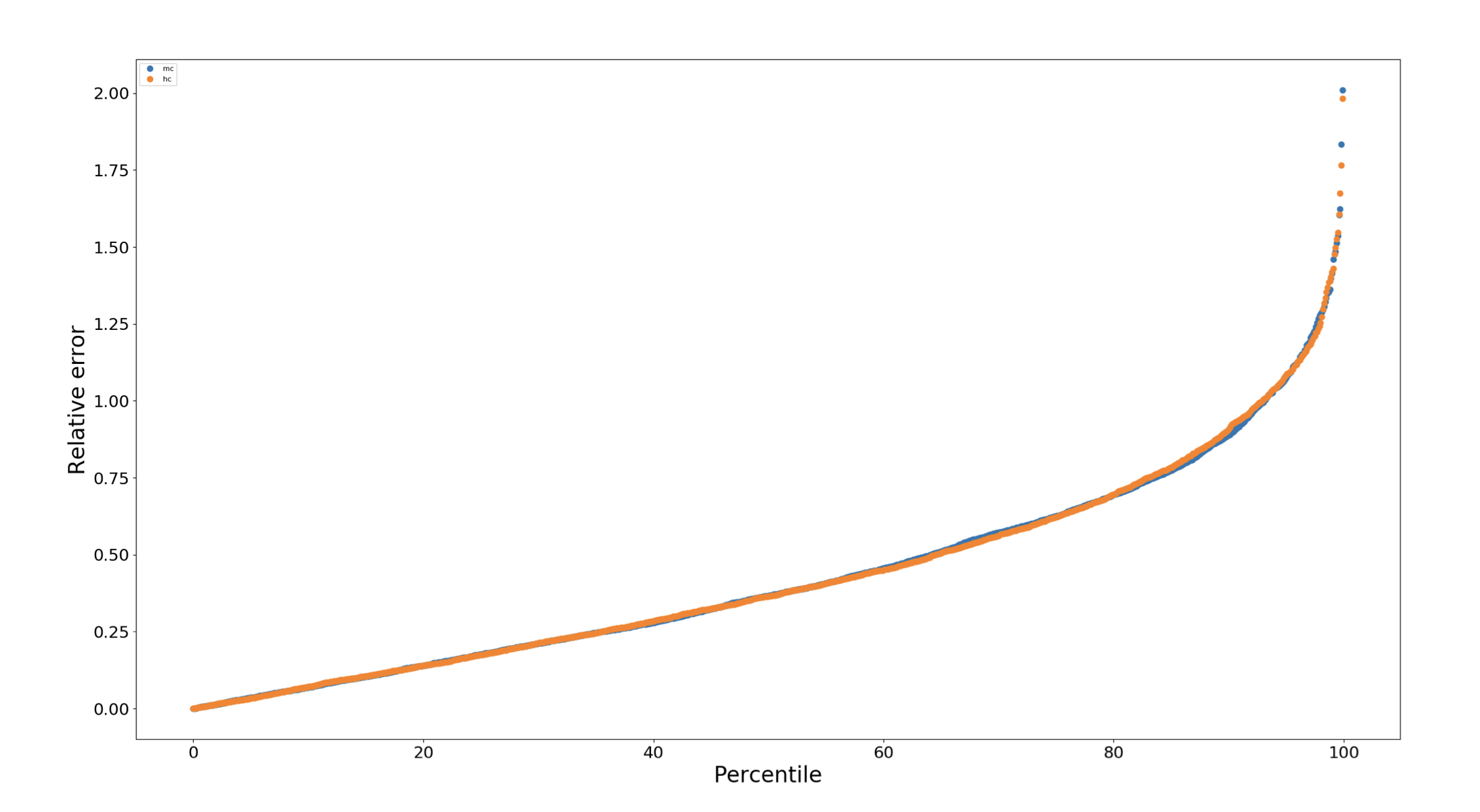
Relative errors of the floating point counter and the Morris++ counter
Hmm. This is interesting, since the relative error of a state-of-the-art algorithm from 2018 has almost the exact same cdf as the relative error of Morris’ original algorithm developed in 1978. This suggested to them that perhaps the original algorithm was in fact asymptotically optimal, but it was the previous analyses of the algorithm which were imperfect.
Nelson and Yu suggest in their paper that even people interested in theory should write a code and run a lot of experiments; they provide the above anecdote as an example.
Proof of optimality
In April 2022 (very recently!), Jelani Nelson and Huacheng Yu published this paper and proved that Morris++ is actually asymptotically optimal. In fact, this paper won the PODS best paper award in 2022. Here’s their main result, which is Theorem 1.1 in their paper, loosely restated according to the notation I used above:
Theorem 1.1. Here, $C$, $C^\prime$, and $C^{\prime\prime}$ will be universal constants. Here, For any $\epsilon, \delta \in \left( 0, \frac{1}{2} \right)$, there is a randomized algorithm for approximate counting which outputs $\tilde{n}$ satisfying:
$\mathbb{P}(\lvert \tilde{n} - n \rvert \geq \epsilon n) < \delta$. Suppose $S$ is such that:
$S > C \left( \log(\log(n)) + \log\left( \frac{1}{\epsilon} \right) + \log\left( \log\left( \frac{1}{\delta} \right) \right) \right)$. Then, letting $M$ denote the required memory in bits, we have the bound:
$\mathbb{P}(M > S) < \exp( -C^\prime \exp(C^{\prime\prime} S))$. Furthermore, this algorithm is asymptotically optimal up to a constant factor: any randomized algorithm which is promised that the final counter is in $\lbrace 1, 2, \cdots, n \rbrace$ has space complexity lower bounded by, with high probability:
$\begin{align*}\Omega\left( \min\left\{ \log(n), \log(\log(n)) + \log\left( \frac{1}{\epsilon} \right) + \log\left( \log\left( \frac{1}{\delta} \right) \right) \right\} \right)\end{align*}$.
The algorithm described by the authors is Morris++ with a general exponent $1 + a$; This is the result we’ve been building up to, and now I’ll give an outline of their proof. For the upper bound, the authors mirror the proof of the Chernoff bound with some additional machinery. First, let $Z_i$ denote the number of increments it takes before the counter increases from $i$ to $i + 1$. Letting $p_i = (1 + a)^{-i}$, notice that $Z_i \sim \operatorname{Geo}(p_i)$ with the following pmf:
\[\mathbb{P}(Z_i = l) = p_i (1 - p_i)^{l-1}.\]Therefore, we have:
\[\mathbb{E}[Z_i] = \frac{1}{p_i} = (1 + a)^i.\]The moment generating function is (summing the geometric series):
\[\mathbb{E}[e^{t Z_i}] = \sum_{l=1}^\infty e^{tl} p_i (1 - p_i)^{l-1} = \frac{p_i e^t}{1 - e^t (1 - p_i)}.\]If $t$ is such that $e^t (1 - p_k) < 1$, an application of Markov’s inequality gives:
\[\begin{align*} \mathbb{P}\left( \sum_{i=0}^k Z_i \geq (1 + \epsilon) \sum_{i=0}^k \frac{1}{p_i} \right) & \leq \exp\left( -t (1 + \epsilon) \sum_{i=0}^k \frac{1}{p_i} \right) \cdot \mathbb{E}\left[ \exp\left( t \sum_{i=0}^k Z_i \right) \right] \\ & = \cdots \\ & = \frac{e^{(k+1) t} (1 + a)^{-\frac{k (k + 1)}{2}}}{\prod_{i=0}^k (1 - e^t (1 - (1 + a)^{-i}))} \cdot \exp\left( -t (1 + \epsilon) \frac{(1 + a)^{k + 1} - 1}{a} \right). \end{align*}\]Then, we choose $t = \ln\left( \frac{1}{1 - \frac{1}{2} \epsilon (1 + a)^{-k}} \right)$, which is a choice that satisfies $e^t (1 - p_k) < 1$. Doing some more algebra with this value of $t$ gives the inequality:
\[\begin{align*} & \frac{e^{(k+1) t} (1 + a)^{-\frac{k (k + 1)}{2}}}{\prod_{i=0}^k (1 - e^t (1 - (1 + a)^{-i}))} \cdot \exp\left( -t (1 + \epsilon) \frac{(1 + a)^{k + 1} - 1}{a} \right) \\ & \quad \leq \exp\left( -\frac{1}{2a} \epsilon (1 + a)^{-k} (1 + \epsilon) ((1 + a)^{k+1} - 1) \right) \cdot \prod_{i=0}^k \frac{1}{1 - \frac{1}{2} \epsilon (1 + a)^{i-k}}. \end{align*}\]Then, we use the inequality $\frac{1}{1 - z} \leq e^{z + z^2}$ for $0 < z < \frac{1}{2}$ for $z \in \mathbb{R}$ and some more algebra gives the bound:
\[\begin{align*} & \exp\left( -\frac{1}{2a} \epsilon (1 + a)^{-k} (1 + \epsilon) ((1 + a)^{k+1} - 1) \right) \cdot \prod_{i=0}^k \frac{1}{1 - \frac{1}{2} \epsilon (1 + a)^{i-k}} \\ & \quad \leq \exp\left( -\frac{1}{4a} \epsilon^2 (1 + a)^{-k} ((1 + a)^{k+1} - 1) \right). \end{align*}\]In particular, when $k > \frac{1}{a}$, we get the bound:
\[\mathbb{P}\left( \sum_{i=0}^k Z_i \geq (1 + \epsilon) \sum_{i=0}^k \frac{1}{p_i} \right) \leq e^{-\frac{\epsilon^2}{8a}}.\]With a symmetric argument, we obtain another bound on the other side:
\[\mathbb{P}\left( \sum_{i=0}^k Z_i \geq (1 - \epsilon) \sum_{i=0}^k \frac{1}{p_i} \right) \leq e^{-\frac{\epsilon^2}{8a}}.\]Nelson and Yu note that this part of the argument can be made shorter (although less elementary) by showing that geometric random variables are sub-gamma. Then, we can use properties of sub-gamma random variables to control $\sum_{i=0}^k Z_i$. As mentioned in the paper, this observation is due to Eric Price.
Therefore, fixing $k > \frac{1}{a}$ as above, with probability at least $1 - e^{-\frac{\epsilon^2}{8a}}$, we have:
\[\left\lvert \sum_{i=0}^k Z_i - \frac{(1 + a)^{k+1} - 1}{a} \right\rvert \leq \epsilon \cdot \frac{(1 + a)^{k+1} - 1}{a}.\]Fixing any $n > \frac{8}{a}$, an application of the union bound tells us that $\frac{(1 + a)^{X_n} - 1}{a}$ is a $(1 \pm 2 \epsilon)$-approximation of $n$ with probability at least $1 - 2 e^{-\frac{\epsilon^2}{8a}}$.
Setting $a = \frac{\epsilon^2}{8 \ln\left( \frac{1}{\delta} \right)}$, this means that the space usage of $\operatorname{Morris}(a)$ is $\log(\log(n)) + 2 \log\left( \frac{1}{\epsilon} \right) + \log\left( \left( \frac{1}{\delta} \right) \right) + O(1)$ bits with high probability. Furthermore, the algorithm outputs a $(1 \pm 2 \epsilon)$-approximation with probability $1 - \frac{2}{\delta}$. Changing constants appropriately, the sharper upper bound on the performance of Morris++ is proven.
On the other hand, the matching lower bound is slightly trickier to prove and uses techniques outside the scope of concentration inequalities and high-dimensional probability. The proof proceeds via a derandomization argument which involves fixing an initial state for all randomness and considering the resulting deterministic algorithm. Then, the authors mirror part of the proof of the pumping lemma for discrete finite automata. For those interested in the details, the original paper is linked above.
Applications
First, Morris’ algorithm spawned a lot more work in the field of random approximation algorithms. For example, the Flajolet-Martin algorithm has a similar structure and famously solves the problem of approximating the number of distinct items in a stream. Morris’ algorithm was also one of the first of many so-called streaming algorithms which produce a sketch, or approximation, to a true value using logarithmically smaller memory.
Sketching and streaming algorithms are used everywhere when working with big data. For example, Google uses algorithms like HyperLogLog++ to provide a sketch of the number of distinct elements for their BigQuery service. As another example, Amazon’s AWS service provides an APPROXIMATE COUNT DISTINCT function to approximate the number of non-null values in a column of data (this is exactly the problem that Morris’ algorithm could solve!). In fact, yet another advantage to Morris’ algorithm is that it can run in an online fashion; it can update its approximate count as we receive more data. This algorithm is really useful!